 LINGCORE SCI
Pseudo-Observations for Survival and Competing-Risk Regression
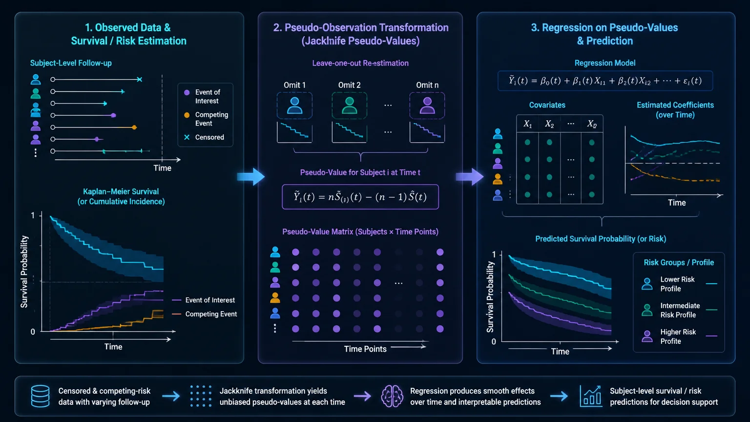
Pseudo-observations convert a censoring-adjusted sample-level survival quantity into subject-indexed quantities that can be modeled with generalized linear or generalized estimating equation methods. They support direct regression of survival probability, restricted mean survival time, cumulative incidence, and selected multi-state probabilities, but their validity still depends on the event estimand, censoring assumptions, time points, and variance estimation.
Clinical researchers often want a quantity that is easy to communicate: survival probability at 12 months, cumulative incidence of relapse by day 180, restricted mean survival time through a prespecified horizon, or the probability of occupying a disease state at a given time. The familiar Cox model does not directly model each of these quantities. It models a relative hazard under a proportional-hazards structure, and the relationship between a hazard ratio and an absolute risk can be difficult to explain when hazards are non-proportional or competing events are common.
Pseudo-observation regression provides another route. A jackknife construction compares the full-sample estimator with leave-one-out estimators. The resulting pseudo-values are indexed by patient and target time, then used as responses in a regression or GEE framework. This lets investigators relate a directly interpretable survival quantity to baseline covariates without pretending that the pseudo-value is a newly observed clinical outcome.
The method is useful because it separates two tasks. First, estimate a censoring-adjusted population quantity such as a Kaplan–Meier survival probability or cumulative incidence. Second, model how that quantity varies with covariates. The separation is also a warning: the regression remains tied to the estimator used to construct the pseudo-values and to the assumptions supporting that estimator.
How pseudo-values are constructed
Let the target parameter be an estimator of a survival-related quantity at time t. The full-sample estimate is obtained from all participants. For participant i, a leave-one-out estimate is obtained after removing that participant. A commonly used jackknife pseudo-value has the form n times the full-sample estimate minus n − 1 times the leave-one-out estimate. The exact notation changes with the target quantity, but the principle is the same: each participant receives a constructed value whose collection preserves the target estimator in an estimating-equation sense.
Pseudo-values can be generated for multiple time points. A long-format data set then contains repeated pseudo-value records for each participant, with a time-point indicator and covariates. GEE or another method accounting for within-participant correlation can estimate covariate effects across the selected time points. The working correlation is a modeling choice, while the sandwich variance is commonly used to account for the dependence created by repeated pseudo-values.
These values should not be described as observed survival times, individual probabilities, or guaranteed unbiased subject-level outcomes. They are estimating constructs. Some may fall outside the usual 0-to-1 range, particularly in finite samples or near the boundary of the estimated survival curve. That behavior is not automatically an error; it reflects the jackknife construction and reinforces the need to interpret model-based predictions rather than isolated pseudo-values.
What can be modeled directly
| Target quantity | Typical estimator | Clinical interpretation |
|---|---|---|
| Survival probability at t | Kaplan–Meier-based pseudo-values under appropriate censoring assumptions. | Probability of remaining event-free beyond a specified time. |
| Restricted mean survival time | Area-under-the-survival-curve estimator followed by pseudo-value regression. | Average event-free time through a prespecified horizon. |
| Cumulative incidence | Cause-specific cumulative-incidence pseudo-values under competing risks. | Probability of experiencing a specified event type by time t in the presence of other event types. |
| State-occupation probability | Multi-state transition-probability or occupation-probability pseudo-values. | Probability of being in a clinically defined state at a specified time. |
The target must be named before the regression model is selected. For example, a covariate effect on cumulative incidence is not the same as a covariate effect on a cause-specific hazard. Similarly, an effect on RMST is not a hazard ratio. Pseudo-observations make direct modeling possible; they do not make different estimands interchangeable.
Pseudo-observations and competing risks
When death or another event prevents the outcome of interest, cumulative incidence is often the clinically relevant target. Pseudo-values can be constructed for the cumulative incidence function and then modeled with covariates. This supports direct statements such as the adjusted difference in the probability of relapse by day 180, provided the competing-event definition and censoring assumptions are clear.
The competing-risk estimand must remain visible in the manuscript. A model for the cumulative incidence of relapse is not automatically a Fine–Gray model, and a pseudo-value regression coefficient should not be labeled a subdistribution hazard ratio unless the fitted model actually estimates that quantity. Investigators should report the event of interest, competing events, administrative censoring, and the time horizon together.
Researchers comparing approaches can consult the site’s guides to competing-risks analysis, restricted mean survival time, and joint frailty models. These methods answer different questions. A pseudo-value model can be useful for direct risk or RMST regression, while a joint frailty model addresses dependence between recurrent and terminal processes.
Choosing the regression layer
Once pseudo-values have been computed, researchers often use a generalized linear model or GEE with a link function chosen for the target quantity. The link should respect the scientific scale and the behavior of the fitted predictions. A complementary-log-log link may be useful for certain survival-probability representations, while identity or other links may be considered for RMST differences. The choice is not a cosmetic software setting; it changes how coefficients map to the target parameter.
For several time points, include time indicators or a prespecified time structure. An interaction between a covariate and time can examine whether an effect varies across the follow-up grid. Do not report a single time-averaged effect if the model allows strong time variation without showing the time-specific results. Conversely, do not test many time points and highlight only the most favorable one without addressing multiplicity and selective reporting.
For non-randomized data, pseudo-observations do not replace confounding control. Covariate adjustment, propensity-score weighting, overlap weighting, or AIPW may be incorporated depending on the causal estimand and design. The pseudo-value layer concerns the outcome quantity; it does not by itself identify a causal effect.
Assumptions and diagnostics
The first assumption is tied to the estimator used to create the pseudo-values. Kaplan–Meier-based quantities require a defensible independent-censoring structure conditional on the variables included in the analysis. If censoring depends on unmeasured prognosis, the pseudo-values do not repair that problem. Left truncation, delayed entry, time-dependent covariates, informative loss to follow-up, and competing events require an estimator and data structure that explicitly address them.
Second, the regression model must be adequate for the target quantity. Inspect fitted survival or cumulative-incidence curves against nonparametric estimates where possible. Examine predictions at clinically relevant time points and check whether they remain in an interpretable range. Report how standard errors were calculated and whether repeated pseudo-values from the same participant were handled in the variance estimator.
Third, time-point selection matters. A dense grid can create highly correlated outcomes and unstable interactions; a sparse grid can miss clinically important changes. Choose time points from the clinical question, event density, and prespecified horizon. If the analysis uses a data-driven grid, explain that choice and assess whether conclusions are sensitive to reasonable alternatives.
| Diagnostic area | Questions to answer | Red flag |
|---|---|---|
| Event definition | What is the event of interest, competing event, and censoring event? | Different sections use different endpoint definitions. |
| Target time | Why were these time points and horizon selected? | Only the most favorable time point is reported. |
| Variance | How were within-subject repeated pseudo-values handled? | Ordinary independent-observation standard errors are used without justification. |
| Prediction | Do predicted survival probabilities, risks, or RMST contrasts remain clinically interpretable? | Predictions are treated as individual observed probabilities. |
| Confounding | What identifies the causal contrast, if a causal claim is made? | Pseudo-value regression is presented as confounding control. |
Five steps for a defensible analysis
| Step | Research action | Quality gate |
|---|---|---|
| 1. Define the estimand | Specify survival probability, RMST, cumulative incidence, or state-occupation probability, along with time horizon and contrast. | The target is stated in absolute or clinically interpretable terms. |
| 2. Map event and censoring processes | Define event of interest, competing events, entry time, administrative censoring, and loss to follow-up. | The estimator used to create pseudo-values matches the observed-data structure. |
| 3. Construct pseudo-values | Use the full-sample and leave-one-out estimators at prespecified time points. | Time-point selection, estimator, and software implementation are documented. |
| 4. Fit and diagnose the regression | Use an appropriate link and GEE or other variance method for repeated pseudo-values. | Predictions, uncertainty, correlation handling, and model fit are reported. |
| 5. Report the clinical scale | Present absolute risks, RMST contrasts, or state probabilities with uncertainty, not only regression coefficients. | The discussion distinguishes association, prognosis, and causal effect. |
Evidence Summary Table
| Source | Contribution | Evidence boundary |
|---|---|---|
| Andersen and Perme, 2010 PubMed record | Reviews pseudo-observations for survival and event-history quantities, including survival probabilities, RMST, cumulative incidence, and multi-state probabilities. | Methodological review; the validity of each application depends on its estimator and censoring structure. |
| Andersen, Hansen, and Klein, 2004 PubMed record | Develops regression analysis of restricted mean survival time based on pseudo-observations. | RMST-specific methods; the time horizon must be prespecified and clinically meaningful. |
| Klein et al., 2008 Open-access article | Describes SAS and R functions for pseudo-values in survival, RMST, and cumulative-incidence regression, with a bone-marrow-transplant illustration. | Implementation guidance; software output does not remove the need for design and estimand checks. |
| Andersen, Klein, and Rosthøj, 2003 Cited methodological source | Introduces generalized linear models for correlated pseudo-observations with applications to multi-state models. | Multi-state extension; transition definitions and within-subject dependence remain central. |
| Event History Regression with Pseudo-Observations, 2022 Journal of Statistical Software | Provides a modern implementation perspective for regression with pseudo-observations in event-history analysis. | Software and methods resource; analysts should verify package assumptions and version-specific behavior. |
How to report the method
A manuscript should name the target parameter, estimator, time points, censoring assumptions, and regression link. State whether pseudo-values were generated for survival, RMST, cumulative incidence, or a multi-state probability. Explain the leave-one-out construction at a level that permits reproduction, and describe how repeated pseudo-values were handled for standard errors.
Results should include the number of participants, events, competing events, and censored observations. Present estimates on the clinical scale whenever possible: survival probabilities, absolute risk differences, RMST differences, or state-occupation probabilities. If a regression coefficient is the primary result, show how it translates into an interpretable contrast at clinically relevant covariate patterns and time points.
Finally, avoid claiming that pseudo-observations make a survival analysis “non-parametric” in every meaningful sense or that they automatically solve censoring, confounding, or competing-risk bias. They are a flexible bridge between censoring-adjusted estimators and regression models. Their credibility depends on a coherent estimand, an appropriate estimator, valid variance handling, and transparent reporting.
Researcher's Toolkit
Use Lingcore SCI to structure and audit time-to-event evidence:
- Paper Analyzer: extract event definitions, censoring rules, time horizons, pseudo-value construction, and reported uncertainty from published studies.
- Review Builder: compare pseudo-observation, Cox, RMST, competing-risk, multi-state, and joint-frailty evidence with source-linked boundaries.
- Journal Matcher: identify journals aligned with survival analysis, clinical trials, outcomes research, and medical biostatistics.
Medical Disclaimer: This article is for research and educational purposes only. It does not provide medical advice, treatment recommendations, or a substitute for protocol-specific statistical review. Researchers must verify methods against the original sources, data structure, estimand, and clinical context before using them in a study or manuscript.